munro | region | height | first_route_title | first_route_url | time_hours_min | time_hours_max | distance_km | ascent | scramble | exposed | spate | bog | river | arete | toilet | bothy | pub | car_park | deer_fence | ascents | rating |
|---|---|---|---|---|---|---|---|---|---|---|---|---|---|---|---|---|---|---|---|---|---|
A' Bhuidheanach Bheag | Cairngorms | 936 | Càrn na Caim and A' Bhuidheanach Bheag from Drumochter | https://www.walkhighlands.co.uk/cairngorms/carn-na-caim.shtml | 5 | 6 | 19 | 824 | false | false | false | true | false | false | false | false | false | false | false | 10,604 | 2.40 |
A' Chailleach (Fannichs) | Ullapool | 997 | Sgùrr Breac and a' Chailleach from near Braemore | https://www.walkhighlands.co.uk/ullapool/sgurrbreac.shtml | 6 | 8 | 16 | 1,127 | false | false | false | true | false | false | false | false | false | false | false | 5,693 | 3.48 |
Munro Tidy Tuesday
I was immediately obsessed when I saw the Tidy Tuesday theme was Scottish Munros - we have climbed 58/282 so far. As I assume is the case for the majority of baggers, we use walkhighlands for all our munro info and routes. walkhighlands is one of the unequivocally wonderful bits of the internet and I can’t believe it’s free. We donate to keep it going, and if you’re a bagger who uses it often, I’d encourage you to do the same. When I saw the Tidy Tuesday dataset, I knew I wanted to try and combine the provided data from the Database of British and Irish Hills v18.2 with what’s available on walkhighlands.
Because I’ve made certain career choices, my day-to-day activity now involves a lot less coding and a lot more admin and I realised I was starting to lose some of my R so this has been a nice excuse to refresh. I’m gearing up for another semester of teaching R to students in the age of AI and it has been interesting to reflect on how I’m using AI myself. Pleasingly, many of the solutions to the many problems I had to solve came from my knowledge of Munros and Gaelic. AI sometimes provided the code but it’s a nice reminder it can only provide the answers to questions you know to ask.
Walkhighlands munro info
The reason I wanted to use walkhighlands data is that it has a bunch of route information that I could use for exploration that wasn’t contained in the Database of British and Irish Hills that is the base of the Tidy Tuesday data:
- Region
- Estimated length of walk in hours
- Distance of walk
- Total ascent of route (not just of each individual Munro)
- Route descriptions
- User rating of each Munro
- Number of ascents recorded for each Munro
I contacted walkhighlands to ask permission to share what I’ve done and they said yes because they’re lovely. I’ve still decided not to include the code I used for web scraping so I don’t inadvertently cause them any issues and so I’ll just describe roughly what I did instead.
The approach was to first scrape walkhighlands for the list of Munros, the region in which they are located, and their height from the Munro A-Z page. Then it took one route for each munro (the first listed), the min and max estimated walk time, distance in km, total ascent in metres, and used regex to look for certain words that describe walk features that might be of interest (scramble, exposed, arete, river, spate, bog). walkhighlands also provides a Grade rating for each walk as well as a bog factor, however, these are represented as images, and try as I (well, AI) might, I could not get it to parse this information.

An important note for those of you who are familiar with walkhighlands, as highlighted, I included one route per munro - the first one listed. This can make a big difference to the walk, for example, which route you take up Ben Nevis significantly changes the fear factor and technicality. Text mining is also a blunt tool and only looks at whether a word is contained in the walk report rather than its context - a route that reads “there is no scrambling required” would still have been included in the “scramble” category and exposure can relate to the weather or heights.
It took a long time to get the AI to provide code that worked and there were a number of issues - at one point it was matching the route to the wrong Munro, then it didn’t return all Munros, then it was missing a bunch of routes. I had to manually create a file of some routes to load in because I could not find a solution as to why these handful were failing. Because I could not have done any of this type of scraping without AI, I really have no idea why it works and why it didn’t. This is intellectually unsatisfying but also, the idea you’d be willing to trust this black box of “knowledge” to something more serious than an obsessive deep dive into your favorite mountains is madness.
Here’s what the walkhighlands data looks like.
Database of British and Irish Hills
Next it was time to load in the Tidy Tuesday dataset which is from the Database of British and Irish Hills. In order to be able to join this with my walkhighlands database, I had to do quite a lot of wrangling although thankfully I was not reliant on AI and mainly able to achieve it because of my existing knowledge of Munros and Gaelic.
I wasn’t that bothered about the Munro status changes over the years as the walkhighlands database allowed me to do other more interesting analyses so I dropped these bits.
Show code
library(tidyverse)
library(fuzzyjoin)
library(ggthemes)
library(ggridges)
library(flextable)
library(stringi)
library(tidytext)
library(sf)
library(plotly)
library(rnaturalearth)

scottish_munros <- readr::read_csv('https://raw.githubusercontent.com/rfordatascience/tidytuesday/main/data/2025/2025-08-19/scottish_munros.csv')

raw_data <- read_csv("https://www.hills-database.co.uk/munrotab_v8.0.1.csv")

scottish_munros <- raw_data |>
  filter(`2021` == "MUN") |>
  select(
    `DoBIH Number`, Name,
    `Height (m)`, xcoord, ycoord, "Grid Ref",
  ) |>
  drop_na(`DoBIH Number`) |>
  rename(
    munro = "Name",
    height = `Height (m)`,
    number = `DoBIH Number`,
    grid_ref = "Grid Ref"
  )
rm(raw_data)
What’s in a name (issues)
The first problem to solve before trying to join the two datasets was that some of the names of the Munros differ between the two - sometimes this is because there are variants in the Gaelic (Carn Eighe/Càrn Eige), sometimes the Anglicised version is used, and sometimes it’s because multiple Munros have the same name so they have additional information added in parenthesis in one of the files (Stuc an Lochain [Stuchd an Lochain]/Stùcd an Lochain).
Show code
scottish_munros <- scottish_munros |>
  # Standardise names in the 'dobih' dataset to Walkhighlands spellings
  mutate(
    munro = case_when(
      munro == "A' Chraileag [A' Chralaig]" ~ "A' Chralaig",
      munro == "Beinn Challuim [Ben Challum]" ~ "Ben Challum",
      munro == "Beinn Sheasgarnaich [Beinn Heasgarnich]" ~ "Beinn Heasgarnich",
      munro == "Beinn a' Bhuird North Top" ~ "Beinn a' Bhùird",
      munro == "Ben Klibreck - Meall nan Con" ~ "Ben Klibreck",
      munro == "Blabheinn [Bla Bheinn]" ~ "Blà Bheinn",
      munro == "Cac Carn Beag (Lochnagar)" ~ "Lochnagar",
      munro == "Carn Eighe" ~ "Càrn Eige",
      munro == "Carn a' Choire Bhoidheach" ~ "Càrn a' Choire Bhòidheach",
      munro == "Creag a' Mhaim" ~ "Creag a'Mhàim",
      munro == "Glas Leathad Mor (Ben Wyvis)" ~ "Ben Wyvis",
      munro == "Leabaidh an Daimh Bhuidhe (Ben Avon)" ~ "Ben Avon",
      munro == "Meall Garbh" ~ "Meall Garbh (Ben Lawers)",
      munro == "Meall na Aighean" ~ "Creag Mhòr (Meall na Aighean)",
      munro == "Sgurr Dearg - Inaccessible Pinnacle" ~ "Inaccessible Pinnacle",
      munro == "Sgurr Mhor (Beinn Alligin)" ~ "Sgùrr Mòr (Beinn Alligin)",
      munro == "Sgurr na h-Ulaidh [Sgor na h-Ulaidh]" ~ "Sgòr na h-Ulaidh",
      munro == "Sgurr nan Ceathramhnan [Sgurr nan Ceathreamhnan]" ~ "Sgùrr nan Ceathreamhnan",
      munro == "Stob Coir' an Albannaich" ~ "Stob Coir an Albannaich",
      munro == "Stuc an Lochain [Stuchd an Lochain]" ~ "Stùcd an Lochain",
      munro == "Càrn nan Gobhar (Strathfarrar)" ~ "Càrn nan Gobhar (Loch Mullardoch)",
      TRUE ~ munro
    )
  )
After standardising the names, to facilitate the join I also had to convert to lower case, remove accents (whether they’re used differs between the datasets), and any parenthesis information from the Munro names.
After this cleaning, because multiple Munros have the same name, I needed to join on height to distinguish them as thankfully, there aren’t two Munros with the same name and height. However, a problem I wasn’t anticipating is that height measurements differed between the datasets. A lot of these can be put down to rounding - walkhighlands uses whole numbers whilst the DoBIH uses two decimal places. However, this doesn’t explain them all (the largest difference is 8.1 metres, that’s a lot!). I don’t know which one is “correct” or why they differ but given DoBIH is numerically more precise, I decided to use that as my measure of height in any analysis.
My AI-fuelled discovery was fuzzyjoin which allows you to set a tolerance level for the join and pick a best match. I’ve never needed this before but it provided itself to be extremely useful - with a bit of trial and error I set a tolerance of 10m and manually checked the output to ensure everything had lined up correctly.
UPDATE: Because walkhighlands are great (honestly go and give them some money), they have updated the heights based on the DoBIH data so they now match (is this impact?).
Show code
# 0) Choose a tolerance in metres (use Inf if you want “nearest regardless”)
tol_m <- 10

# 1) Normalise names in BOTH tables: remove (...) and [...], drop accents, lower-case, squish
x <- walkhighlands %>%
  mutate(
    munro_key = munro %>%
      str_replace_all("\\s*\\([^)]*\\)", "") %>%   # remove text in ( )
      str_replace_all("\\s*\\[[^\\]]*\\]", "") %>% # remove text in [ ]
      stri_trans_general("Latin-ASCII") %>%
      str_to_lower() %>%
      str_squish(),
    height = parse_number(as.character(height)),
    row_id_x = row_number()
  )

y <- scottish_munros %>%
  mutate(
    munro_key = munro %>%
      str_replace_all("\\s*\\([^)]*\\)", "") %>%
      str_replace_all("\\s*\\[[^\\]]*\\]", "") %>%
      stri_trans_general("Latin-ASCII") %>%
      str_to_lower() %>%
      str_squish(),
    height = parse_number(as.character(height)),
    row_id_y = row_number()
  )

# 2) Fuzzy FULL join on exact munro_key + height within tolerance
candidates <- fuzzy_full_join(
  x, y,
  by = c("munro_key" = "munro_key", "height" = "height"),
  match_fun = list(`==`, function(a, b) abs(a - b) <= tol_m)
) %>%
  # standardise suffixes for older fuzzyjoin that uses .x/.y
  rename_with(~ str_replace(.x, "\\.x$", "_wh")) %>%
  rename_with(~ str_replace(.x, "\\.y$", "_dobih")) %>%
  mutate(
    height_diff = abs(height_wh - height_dobih),
    height_diff = if_else(is.na(height_diff), Inf, height_diff)
  )

# 3) Reduce to one nearest match per row on each side, preserving FULL-join behaviour
best_for_left  <- candidates %>%
  group_by(row_id_x) %>%
  slice_min(height_diff, with_ties = FALSE) %>%
  ungroup()
best_for_right <- candidates %>%
  group_by(row_id_y) %>%
  slice_min(height_diff, with_ties = FALSE) %>%
  ungroup()

munro_dat <- bind_rows(best_for_left, best_for_right) %>%
  distinct(row_id_x, row_id_y, .keep_all = TRUE) %>%
  mutate(
    site_key = coalesce(grid_ref, paste0(xcoord, "_", ycoord)),
    munro_wh_clean = str_replace(munro_wh, "\\s*\\([^)]*\\)$", "")  # drop "(Loch Mullardoch)" etc.
  ) %>%
  group_by(site_key) %>%
  slice_min(height_diff, with_ties = FALSE) %>%   # keep the single closest pair for that site
  ungroup() %>%
  mutate(munro_wh = munro_wh_clean) %>%
  select(-munro_wh_clean) |>
  mutate(time = (time_hours_min + time_hours_max) / 2) |>
  select(-munro_dobih,-munro_key_dobih) |>
  rename(munro = munro_wh)|>
  mutate(scramble_exposed = case_when(
    scramble & exposed ~ "Both",
    scramble & !exposed ~ "Scramble",
    !scramble & exposed ~ "Exposed",
    TRUE ~ "Neither"
  )) |>
  mutate(scramble_exposed = factor(scramble_exposed,
                                   levels = c("Neither", "Scramble", "Exposed", "Both"))) |>
    mutate(wet = case_when(
    spate & bog ~ "Both",
    spate & !bog ~ "Large river",
    !spate & bog ~ "Boggy",
    TRUE ~ "Neither"
  )) |>
  mutate(wet = factor(wet,
                                   levels = c("Neither", "Large river", "Boggy", "Both")))


rm(x,y, best_for_left, best_for_right, candidates, tol_m, walkhighlands, scottish_munros)
I also created some manual colour scales on a nature theme:
Show code
nature_6 <- c(
  "#355E3B",
  "#4B4F58",
  "#4682B4",
  "#8E6C88",
  "#E07B39",
  "#BDB76B"
)

nature_5 <- c(
  "#355E3B",
  "#4B4F58",
  "#4682B4",
  "#E07B39",
  "#BDB76B"
)

nature_4 <- c(
  "#355E3B",
  "#4B4F58",
  "#4682B4",
  "#E07B39"
)

nature_13 <- c(
  "#355E3B",  # Pine green
  "#6B8E23",  # Moss
  "#BDB76B",  # Dry grass
  "#8B5A2B",  # Earth brown
  "#D2B48C",  # Sand
  "#87CEEB",  # Sky blue
  "#4682B4",  # Loch blue
  "#191970",  # Mountain shadow (midnight blue)
  "#7D7D7D",  # Granite grey
  "#A9A9A9",  # Slate grey
  "#8E6C88",  # Heather purple
  "#E07B39",  # Sunset orange
  "#FFD700"   # Sun yellow
)
Routes vs Munros
For some of the analyses later on, it makes more sense to do the analysis by route rather than by individual mountains - one route can have multiple Munros and the time, distance, and total ascent is for the entire route, not individually.
There are 282 Munros, but these are covered by 152 walkhighlands routes.
Because the user ratings and number of ascents are done by individual Munro rather than route, I also had to calculate the average for these for the route. It won’t be completely accurate because you don’t have to climb all the Munros on a given route, but given that I am just dicking about on the internet, that’s probably fine.
Show code
route_dat <-munro_dat |>
  select(first_route_url, first_route_title,
         region, time_hours_min:deer_fence, time, scramble_exposed, wet) |>
  unique()

route_stats <- munro_dat |>
  group_by(first_route_url) |>
  summarise(route_rating = janitor::round_half_up(mean(rating), 2),
            route_ascents = janitor::round_half_up(mean(ascents),0 ))

route_dat <- route_dat |>
  left_join(route_stats)
Scrambling and exposure
I have a reasonably bad fear of heights so anything that mentions scrambling or exposure worries me. First question, are higher munros scarier?
Big thank you to Jessica Moore for the inspiration for this one.
Show code
ggplot(munro_dat,
       aes(height_dobih, scramble_exposed, fill = scramble_exposed)) +
  geom_density_ridges(quantile_lines = TRUE, quantile_fun = mean,
                      vline_linetype = "dashed",
                      aes(color = "Mean height (m)")) +
  scale_y_discrete(expand = c(0.01, 0)) +
  scale_x_continuous(expand = c(0.01, 0)) +
  scale_color_manual(values = c("Mean height (m)" = "black")) +
  theme_economist() +
  scale_fill_manual(values = nature_4) +
  labs(x = NULL, y = NULL,
       title = "Are higher Munros scarier?",
       colour = NULL,
       subtitle = "Routes descriptions that mention exposure tend to be on higher Munros")+
  guides(fill = "none") +
  theme(legend.position = "bottom",
        legend.position.inside = c(0.8,0.10))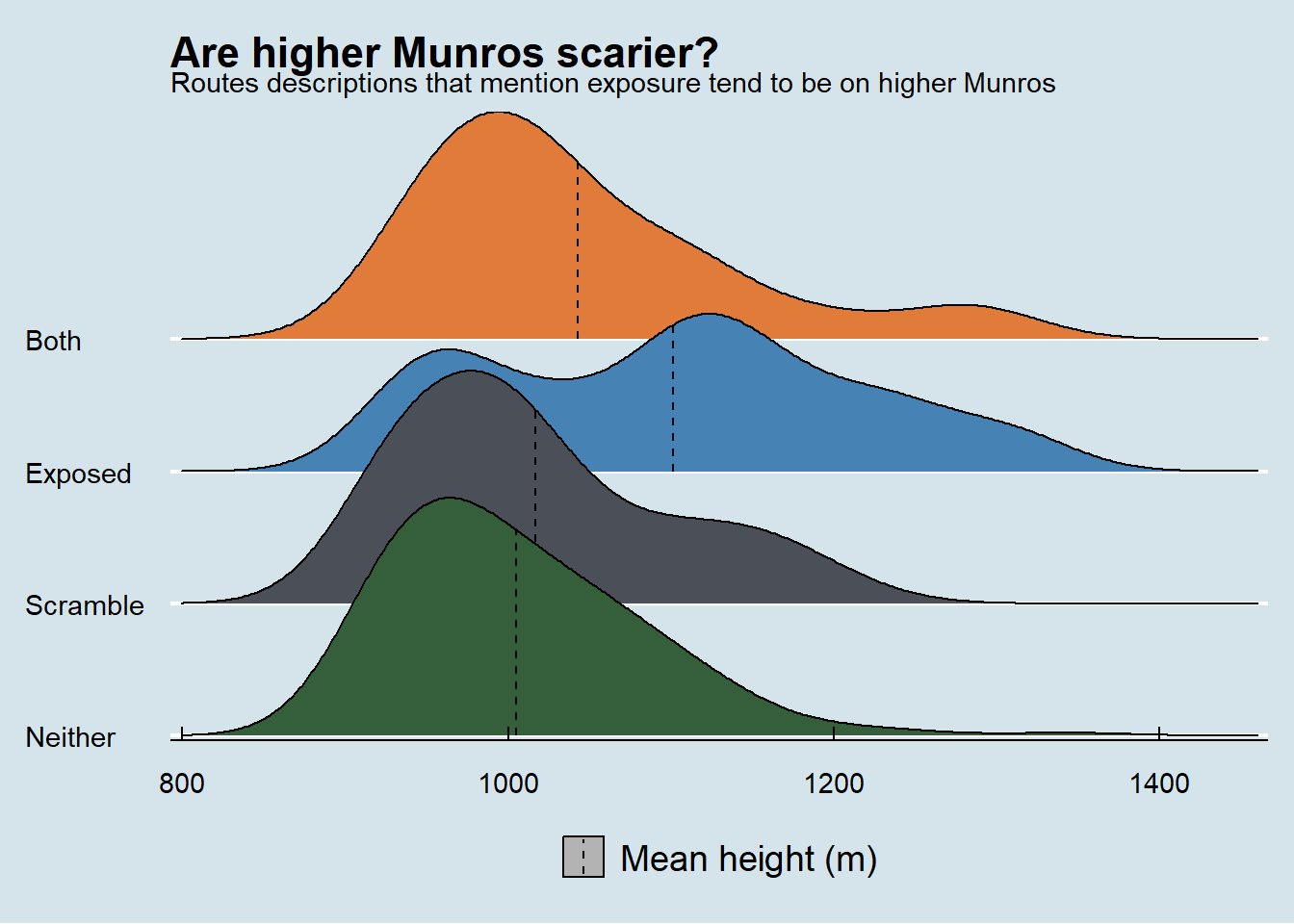
For locating the scary munros, I decided that an interactive plotly map was called for so that you can easily isolate the different types - these work much better on a full browser than a phone.
Have I mentioned that I dislike heights and exposure?
Show code
munros_map <- munro_dat %>%
  select(munro, region, xcoord, ycoord, height_dobih, scramble_exposed, wet, toilet, pub, bothy, deer_fence, car_park) %>%
  na.omit()

# Convert OSGB36 coordinates to sf object
munros_sf <- munros_map %>%
  st_as_sf(coords = c("xcoord", "ycoord"),
           crs = 27700)  # EPSG:27700 is OSGB36 / British National Grid

# Transform to WGS84 (lat/long) for easier plotting
munros_lat_long <- munros_sf %>%
  st_transform(crs = 4326)

# Extract coordinates for ggplot
munros_coords <- munros_lat_long %>%
  mutate(
    longitude = st_coordinates(.)[,1],
    latitude = st_coordinates(.)[,2]
  ) %>%
  st_drop_geometry() %>%
  arrange(-height_dobih)


uk_map <- rnaturalearth::ne_countries(scale = "large",
                                  country = "United Kingdom",
                                    returnclass = "sf")

# Step 2: Specify shape codes (16 = circle, 17 = triangle, etc.)
shape_values <- c(
  "Neither" = 16,    # filled circle
  "Scramble" = 17,   # filled triangle
  "Exposed" = 15,    # filled square
  "Both" = 18        # filled diamond
)

p <- ggplot() +
  geom_sf(data = uk_map, fill = "lightgray", color = "darkgrey", size = 0.3) +
  coord_sf(xlim = c(-8, -1.5), ylim = c(56.5, 58.6)) +
  geom_jitter(data = munros_coords,
             aes(x = longitude,
                 y = latitude,
                 shape = scramble_exposed,
                 colour = scramble_exposed,
                 text = munro),
             size = 1,
             height = .05,
             width = .05) +
  scale_x_continuous(breaks = NULL) +
  scale_shape_manual(values = shape_values) +
  scale_y_continuous(breaks = NULL) +
  scale_colour_manual(values = nature_4) +
  labs(title = "Where are the scary Munros?",
       subtitle = "Walk descriptions that reference:",
       colour = "Route mentions", shape = "Route mentions") +
  theme_economist() +
  theme(
    axis.text = element_blank(),
    axis.ticks = element_blank(),
    axis.title = element_blank(),
    panel.grid = element_blank(),
    panel.border = element_blank(),
    legend.text = element_text(size = 10)
  )

ggplotly(p, tooltip = "text")
By region
I also thought it would be fun to look into regional differences. The munros vary massively in character depending on where you are in the country (you can imagine hobbits living in Cairngorms whilst Skye would be home to dragons), but how is this reflected in the walk features?
Regional map
Which Munros are in which region is taken from the walkhighlands A-Z but I’ve had a few people ask since posting this, so here’s an easy to read map.
Show code
p3 <- ggplot() +
  geom_sf(data = uk_map, fill = "lightgray", color = "darkgrey", size = 0.3) +
  coord_sf(xlim = c(-8, -1.5), ylim = c(56.5, 58.6)) +
  geom_jitter(data = munros_coords,
             aes(x = longitude,
                 y = latitude,
                 colour = region,
                 text = munro),
             size = 1,
             height = .05,
             width = .05) +
  scale_x_continuous(breaks = NULL) +
  scale_y_continuous(breaks = NULL) +
  scale_colour_manual(values = nature_13) +
  labs(title = "Munros by region",
       colour = NULL) +
  theme_economist() +
  theme(
    axis.text = element_blank(),
    axis.ticks = element_blank(),
    axis.title = element_blank(),
    panel.grid = element_blank(),
    panel.border = element_blank(),
    legend.text = element_text(size = 10)
  )

ggplotly(p3, tooltip = "text")
And here’s the counts for how many Munros and routes are in each region. It’s highly correlated, but the ranks do change a little.
Show code
munro_region <- munro_dat |>
  count(region, sort = TRUE) |>
  rename("munros" = "n")

route_region <- route_dat |>
  count(region, sort = TRUE) |>
  rename("routes" = "n")

inner_join(munro_region, route_region) |>
  flextable()|>
  autofit()
region | munros | routes |
|---|---|---|
Fort William | 67 | 38 |
Cairngorms | 54 | 32 |
Perthshire | 28 | 16 |
Kintail | 24 | 10 |
Ullapool | 24 | 9 |
Argyll | 19 | 13 |
Loch Ness | 17 | 7 |
Torridon | 17 | 12 |
Loch Lomond | 14 | 9 |
Isle of Skye | 12 | 10 |
Angus | 3 | 2 |
Sutherland | 2 | 2 |
Isle of Mull | 1 | 1 |
Tallest Munros
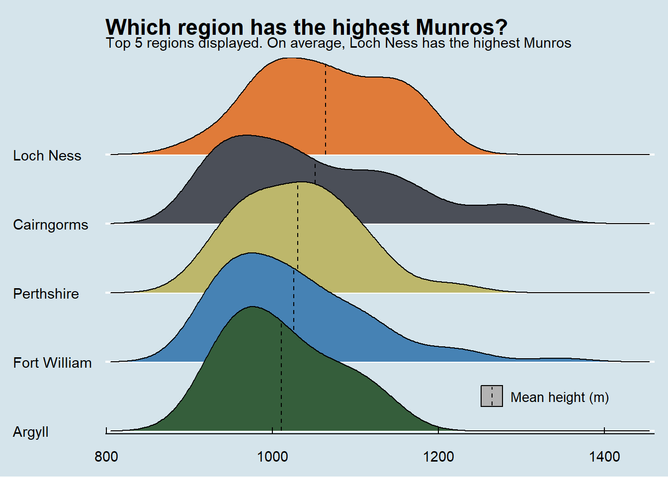
Which region has the tallest Munros?
Show code
region_height <- munro_dat |>
  group_by(region) |>
  summarise(avg_height = mean(height_dobih, na.rm = TRUE), .groups = "drop") |>
  slice_max(avg_height, n = 5)

ggplot(
  semi_join(munro_dat, region_height, by = "region"),
  aes(
    x = height_dobih,
    y = fct_reorder(region, height_dobih, .fun = mean, .desc = FALSE),
    fill = region
  )
)  +
  geom_density_ridges(
    quantile_lines = TRUE, quantile_fun = mean,
    vline_linetype = "dashed",
    aes(colour = "Mean height (m)")
  ) +
  scale_y_discrete(expand = c(0.01, 0)) +
  scale_x_continuous(expand = c(0.01, 0)) +
  scale_colour_manual(values = c("Mean height (m)" = "black")) +
  theme_economist() +
  scale_fill_manual(values = nature_5) +
  labs(
    x = NULL, y = NULL,
    title = "Which region has the highest Munros?",
    colour = NULL,
    subtitle = "Top 5 regions displayed. On average, Loch Ness has the highest Munros"
  ) +
  guides(fill = "none") +
  theme(
    legend.position = "inside",
   legend.position.inside = c(0.8, 0.1),
    legend.text = element_text(size = 10)
  )
And fere’s the full list in table form:
Show code
munro_dat |>
  group_by(region) |>
  summarise(avg_height = mean(height_dobih, na.rm = TRUE), .groups = "drop") |>
  arrange(desc(avg_height)) |>
  flextable() |>
  colformat_double(digits = 0)|>
  autofit()
region | avg_height |
|---|---|
Loch Ness | 1,064 |
Cairngorms | 1,052 |
Perthshire | 1,031 |
Fort William | 1,026 |
Argyll | 1,011 |
Kintail | 1,004 |
Loch Lomond | 989 |
Ullapool | 986 |
Torridon | 979 |
Isle of Mull | 966 |
Isle of Skye | 953 |
Sutherland | 945 |
Angus | 938 |
Longest routes
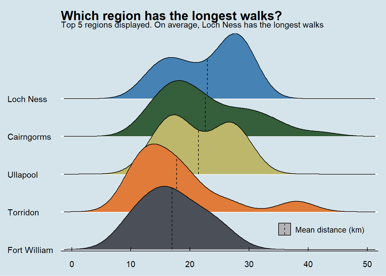
Which region has the longest routes on average by distance?
This plot uses the route data although I am pleased that the order remains the same if you use the munro data (because I only realised I should do it by route after I shared this publicly).
Show code
# Top 5 regions by mean distance
region_distance <- route_dat |>
  group_by(region) |>
  summarise(avg_distance = mean(distance_km, na.rm = TRUE), .groups = "drop") |>
  slice_max(avg_distance, n = 5)

# Keep only those regions in the raw data
top_dat <- semi_join(route_dat, region_distance, by = "region")


ggplot(
  top_dat,
  aes(
    x = distance_km,  # use the per-route variable here
    y = fct_reorder(region, distance_km, .fun = mean, .desc = FALSE),
    fill = region
  )
) +
  geom_density_ridges(
    quantile_lines = TRUE, quantile_fun = mean,
    vline_linetype = "dashed",
    aes(colour = "Mean distance (km)")
  ) +
  scale_y_discrete(expand = c(0.01, 0)) +
  scale_x_continuous(expand = c(0.01, 0)) +
  scale_colour_manual(values = c("Mean distance (km)" = "black")) +
  theme_economist() +
  scale_fill_manual(values = nature_5) +
  labs(
    x = NULL, y = NULL,
    title = "Which region has the longest walks?",
    colour = NULL,
    subtitle = "Top 5 regions displayed. On average, Loch Ness has the longest walks"
  ) +
  guides(fill = "none") +
  theme(
    legend.position = "inside",
    legend.position.inside = c(0.82, .1),
    legend.text = element_text(size = 10)
    )
And here’s the full list in table form:
Show code
route_dat |>
  group_by(region) |>
  summarise(avg_distance = mean(distance_km, na.rm = TRUE), .groups = "drop") |>
  arrange(desc(avg_distance)) |>
  flextable() |>
  colformat_double(digits = 2)|>
  autofit()
region | avg_distance |
|---|---|
Loch Ness | 22.96 |
Cairngorms | 22.59 |
Ullapool | 21.44 |
Torridon | 17.73 |
Fort William | 16.99 |
Perthshire | 16.30 |
Argyll | 16.23 |
Angus | 16.00 |
Kintail | 15.80 |
Loch Lomond | 13.00 |
Sutherland | 10.88 |
Isle of Skye | 10.85 |
Isle of Mull | 9.25 |
Most ascent
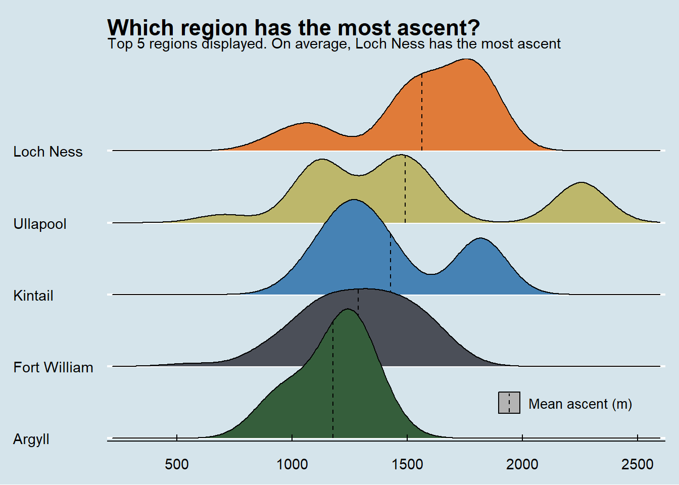
Which region has the most ascent per route?
Again the order doesn’t change if you use routes or Munros as the data (the exact values do slightly but not the rank).
Show code
# Top 5 regions by mean distance
region_ascent <- munro_dat |>
  group_by(region) |>
  summarise(avg_ascent = mean(ascent, na.rm = TRUE), .groups = "drop") |>
  slice_max(avg_ascent, n = 5)

# Keep only those regions in the raw data
top_ascent <- semi_join(munro_dat, region_ascent, by = "region")


ggplot(
  top_ascent,
  aes(
    x = ascent,  # use the per-route variable here
    y = fct_reorder(region, ascent, .fun = mean, .desc = FALSE),
    fill = region
  )
) +
  geom_density_ridges(
    quantile_lines = TRUE, quantile_fun = mean,
    vline_linetype = "dashed",
    aes(colour = "Mean ascent (m)")
  ) +
  scale_y_discrete(expand = c(0.01, 0)) +
  scale_x_continuous(expand = c(0.01, 0)) +
  scale_colour_manual(values = c("Mean ascent (m)" = "black")) +
  theme_economist() +
  scale_fill_manual(values = nature_5) +
  labs(
    x = NULL, y = NULL,
    title = "Which region has the most ascent?",
    colour = NULL,
    subtitle = "Top 5 regions displayed. On average, Loch Ness has the most ascent"
  ) +
  guides(fill = "none") +
  theme(
    legend.position = "inside",
    legend.position.inside = c(0.82, .1),
    legend.text = element_text(size = 10)
    )
And here’s the full list in table form:
Show code
route_dat |>
  group_by(region) |>
  summarise(avg_ascent = mean(ascent, na.rm = TRUE), .groups = "drop") |>
  arrange(desc(avg_ascent)) |>
  flextable() |>
  colformat_double(digits = 0)|>
  autofit()
region | avg_ascent |
|---|---|
Loch Ness | 1,479 |
Ullapool | 1,314 |
Kintail | 1,289 |
Fort William | 1,261 |
Argyll | 1,158 |
Torridon | 1,105 |
Loch Lomond | 1,080 |
Isle of Skye | 1,042 |
Perthshire | 969 |
Cairngorms | 950 |
Isle of Mull | 945 |
Sutherland | 938 |
Angus | 758 |
Munros per route
Where do you get the most bang for your buck?
Show code
munro_dat |>
  count(region, first_route_title, name = "n") |>
  group_by(region) |>
  summarise(avg_count = mean(n), .groups = "drop") |>
  ggplot(aes(
    x = fct_reorder(region, avg_count),
    y = avg_count,
    fill = region
  )) +
  geom_col() +
  scale_fill_manual(values = nature_13) +
  coord_flip() +
  guides(fill = "none") +
  labs(x = NULL, y = "Number of Munros",
       title = "Average number of Munros bagged per route") +
  theme_economist()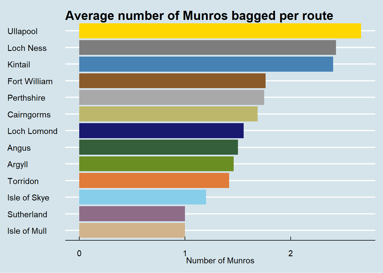
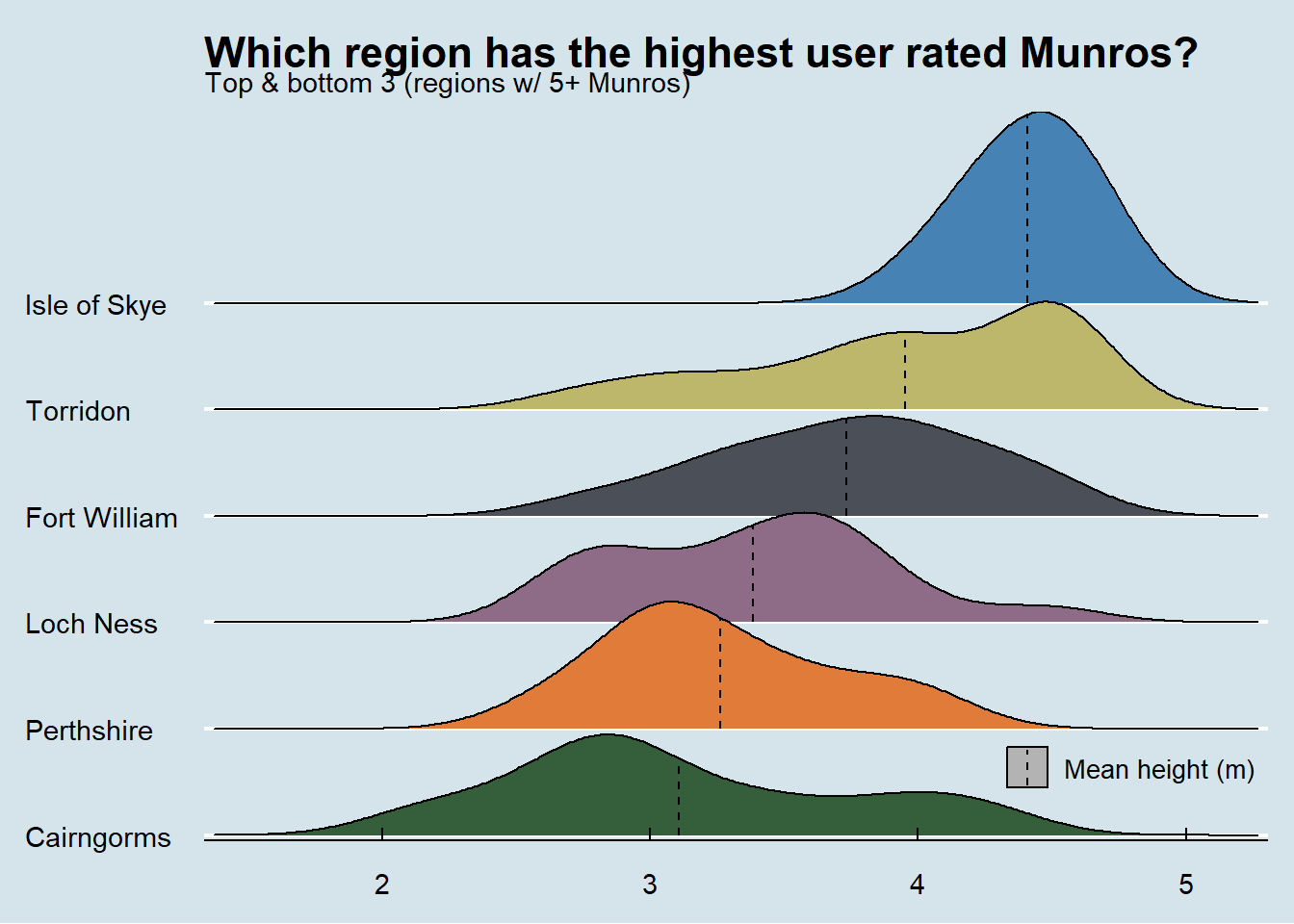
User ratings
Which region has the highest and lowest rated Munros (by user rating)?
Show code
region_rating_top <- munro_dat |>
  group_by(region) |>
  summarise(avg_rating = mean(rating, na.rm = TRUE),
            n = n(),
            .groups = "drop") |>
  filter(n >= 5)|>
  slice_max(avg_rating, n = 3)

# bottom 3

region_rating_bottom <- munro_dat |>
  group_by(region) |>
  summarise(avg_rating = mean(rating, na.rm = TRUE),
            n = n(),
            .groups = "drop") |>
  filter(n >= 5)|>
  slice_min(avg_rating, n = 3)

region_top_bottom <-bind_rows(region_rating_top, region_rating_bottom)

ggplot(
  semi_join(munro_dat, region_top_bottom, by = "region"),
  aes(
    x = rating,
    y = fct_reorder(region, rating, .fun = mean, .desc = FALSE),
    fill = region
  )
)  +
  geom_density_ridges(
    quantile_lines = TRUE, quantile_fun = mean,
    vline_linetype = "dashed",
    aes(colour = "Mean height (m)")
  ) +
  scale_y_discrete(expand = c(0.01, 0)) +
  scale_x_continuous(expand = c(0.01, 0)) +
  scale_colour_manual(values = c("Mean height (m)" = "black")) +
  theme_economist() +
  scale_fill_manual(values = nature_6) +
  labs(
    x = NULL, y = NULL,
    title = "Which region has the highest user rated Munros?",
    colour = NULL,
    subtitle = "Top & bottom 3 (regions w/ 5+ Munros)"
  ) +
  guides(fill = "none") +
  theme(
    legend.position = "inside",
   legend.position.inside = c(0.87, 0.1),
    legend.text = element_text(size = 10)
  )
And here’s the full list in table form:
Show code
munro_dat |>
  group_by(region) |>
  summarise(avg_rating = mean(rating, na.rm = TRUE),
            "no. munros" = n(),.groups = "drop") |>
  arrange(desc(avg_rating)) |>
  flextable() |>
  colformat_double(digits = 2)|>
  autofit()
region | avg_rating | no. munros |
|---|---|---|
Isle of Skye | 4.41 | 12 |
Isle of Mull | 4.07 | 1 |
Torridon | 3.95 | 17 |
Fort William | 3.73 | 67 |
Kintail | 3.69 | 24 |
Ullapool | 3.67 | 24 |
Sutherland | 3.57 | 2 |
Argyll | 3.52 | 19 |
Loch Lomond | 3.44 | 14 |
Loch Ness | 3.38 | 17 |
Perthshire | 3.26 | 28 |
Angus | 3.25 | 3 |
Cairngorms | 3.11 | 54 |
Ascents by rating
Number of ascents (how many people have recorded on walkhighlands that they have summitted a particular Munro) by ratings
Show code
ggplot(route_dat, aes(x = route_ascents, y = route_rating)) +
  geom_point(aes(text = first_route_url)) +
  theme_economist() +
  scale_y_continuous(breaks = seq(1:5)) +
  coord_cartesian(ylim = c(1,5)) +
  labs(y = "User rating (1-5)",
       x = "Number of recorded ascents",
       title = "Number of ascents by rating")+
  annotate(geom = "curve",
          x = 31000, y = 3,
          xend = 31800, yend = 3.75,
          curvature = 0.3,
          arrow = arrow(length = unit(0.5, "lines"))) +
    annotate("text",
           x = 31000, y = 2.8,
           label = "Ben Lomond")+
  annotate(geom = "curve",
          x = 23000, y = 1.45,
          xend = 18900, yend = 2.30,
          curvature = -0.3,
          arrow = arrow(length = unit(0.5, "lines"))) +
    annotate("text",
           x = 28000, y = 1.45,
           label = "The Cairnwell Munros") +
  annotate(geom = "curve",
          x = 5559, y = 1.5,
          xend = 5559, yend = 4.61,
          curvature = -0.55,
          arrow = arrow(length = unit(0.5, "lines"))) +
    annotate("text",
           x = 7600, y = 1.35,
           label = "Sgùrr nan Gillean")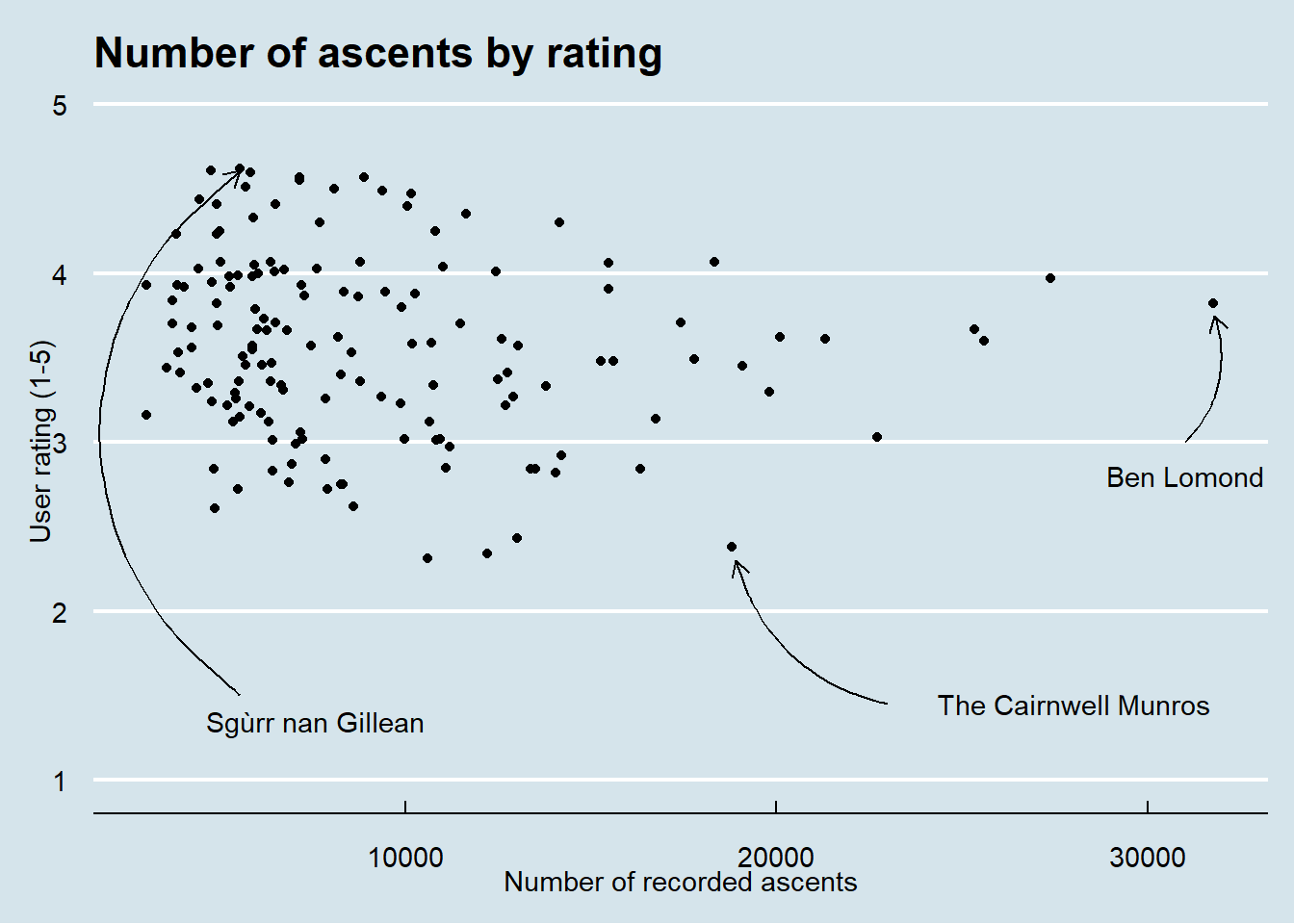
And then as an interactive plot:
Show code
p5 <- ggplot(route_dat, aes(x = route_ascents, y = route_rating)) +
geom_point(aes(text = first_route_title)) +
theme_economist() +
scale_y_continuous(breaks = seq(1:5)) +
coord_cartesian(ylim = c(1,5)) +
labs(y = "User rating (1-5)",
x = "Number of recorded ascents",
title = "Number of ascents per route by rating")
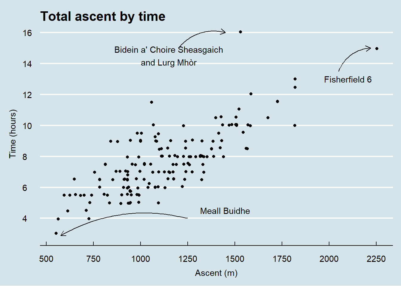
ggplotly(p5)Ascent (m)
As you would expect, total ascent correlates strongly with total time, but there are some points of interest. Bidein a’ Choire Sheasgaich and Lurg Mhòr have the longest estimated walk time but their remoteness means that they’re an outlier in terms of the amount of ascent you’d expect for that time. The Fisherfield 6 claim the prize for most ascent by some distance but are bang on in terms of the ascent/time relationship. Meall Buidhe wins the award for being the quickest munro to bag, with the least ascent.
Show code
ggplot(route_dat, aes(x = ascent, y = time)) +
  geom_jitter(height = .05, width = .05) +
  scale_x_continuous(breaks = seq(500, 2500, 250)) +
  scale_y_continuous(breaks = seq(0, 20, 2)) +
  annotate(geom = "curve",
          x = 1200, y = 15,
          xend = 1450, yend = 16,
          curvature = -0.3,
          arrow = arrow(length = unit(0.5, "lines"))) +
    annotate("text",
           x = 1150, y = 14.5,
           label = "Bidein a' Choire Sheasgaich\nand Lurg Mhòr") +
    annotate(geom = "curve",
          x = 2050, y = 13.5,
          xend = 2220, yend = 15,
          curvature = -0.3,
          arrow = arrow(length = unit(0.5, "lines"))) +
    annotate("text",
           x = 2100, y = 13,
           label = "Fisherfield 6")+
    annotate(geom = "curve",
          xend = 575, yend = 2.9,
          x = 1250, y = 4,
          curvature = 0.2,
          arrow = arrow(length = unit(0.5, "lines"))) +
    annotate("text",
           x = 1450, y = 4.5,
           label = "Meall Buidhe")+
  theme_economist()  +
  labs(x = "Ascent (m)",
       y = "Time (hours)",
       title = "Total ascent by time") +
    theme(legend.position = "inside",
    axis.title.x = element_text(margin = margin(t = 8)),
    axis.title.y = element_text(margin = margin(r = 8)),
    legend.position.inside = c(0.9, .2),
    legend.text = element_text(size = 10)
  )
And here’s an interactive version of that plot that adds in scrambling and exposure because had I mentioned, I am scared of heights.
Show code
p1 <- ggplot(route_dat, aes(x = ascent, y = time)) +
  geom_jitter(aes(shape = scramble_exposed,
                 colour = scramble_exposed,
                 text = first_route_title),
             size = 1) +
  scale_x_continuous(breaks = seq(500,2500, 250)) +
  scale_y_continuous(breaks = seq(0,20,2)) +
  scale_shape_manual(values = shape_values) +
  scale_colour_manual(values= nature_4) +
  labs(x = "Ascent (m)",
       y = "Time (hours)",
       title = "Ascent by time",
       shape = "Route mentions",
       colour = "Route mentions") +
  theme_economist() +
  theme(
    axis.title.x = element_text(margin = margin(t = 8)),
    axis.title.y = element_text(margin = margin(r = 8)),
    legend.text = element_text(size = 10)
  )

ggplotly(p1, tooltip = "text")
Where’s wet?
If the text-mining for scrambling and exposure is a blunt tool then my approach here is even blunter. There are multiple words I could have searched for regarding the presence of water - river, stream, burn - but many of those represent features that don’t make a difference to the walk if they present no difficulty (“cross the bridge over the river”). I decided to use the word “spate” because when the river is large, walkhighlands often highlights that it would be difficult or impossible to cross “in spate”.
So these aren’t all the rivers, just ones where the description indicates crossing them might present an issue.
Show code
shape_values <- c(
  "Neither" = 16,    # filled circle
  "River" = 17,   # filled triangle
  "Boggy" = 15,    # filled square
  "Both" = 18        # filled diamond
)

p2 <- ggplot() +
  geom_sf(data = uk_map, fill = "lightgray", color = "darkgrey", size = 0.3) +
  coord_sf(xlim = c(-8, -1.5), ylim = c(56.5, 58.6)) +
  geom_jitter(data = munros_coords,
             aes(x = longitude,
                 y = latitude,
                 shape = wet,
                 colour = wet,
                 text = munro),
             size = 1,
             height = .05,
             width = .05) +
  scale_x_continuous(breaks = NULL) +
  scale_shape_manual(values = shape_values) +
  scale_y_continuous(breaks = NULL) +
  scale_colour_manual(values = nature_4) +
  guides(shape = "none") +
  labs(title = "Where is wet?\n(Everywhere, it's Scotland)",
              subtitle = "Walk descriptions that reference:",
       colour = "Route mentions", shape = "Route mentions") +
  theme_economist() +
  theme(
    axis.text = element_blank(),
    axis.ticks = element_blank(),
    axis.title = element_blank(),
    panel.grid = element_blank(),
    panel.border = element_blank(),
    legend.text = element_text(size = 10)
  )

ggplotly(p2, tooltip = "text")
Non-natural features
With the usual caveats about the limits of text mining, here’s some maps showing route descriptions that mention non-natural features (bothy, deer fence (because they’re scary), pub, toilet). Some of these are more useful than others.
Bothy
Show code
bothy_plot <- ggplot() +
  geom_sf(data = uk_map, fill = "lightgray", color = "darkgrey", size = 0.3) +
  coord_sf(xlim = c(-8, -1.5), ylim = c(56, 58.6)) +
  geom_jitter(data = filter(munros_coords, bothy == TRUE),
             aes(x = longitude,
                 y = latitude,
                 colour = bothy,
                 text = munro),
             size = 1) +
  scale_x_continuous(breaks = NULL) +
  scale_y_continuous(breaks = NULL) +
  labs(title = "Routes that mention a bothy") +
  guides(colour = "none") +
  theme_economist() +
  theme(
    axis.text = element_blank(),
    axis.ticks = element_blank(),
    axis.title = element_blank(),
    panel.grid = element_blank(),
    panel.border = element_blank(),
    legend.text = element_text(size = 10)
  )

ggplotly(bothy_plot, tooltip = "text")
Deer fences
I really hate deer fences.
Show code
fence_plot <- ggplot() +
  geom_sf(data = uk_map, fill = "lightgray", color = "darkgrey", size = 0.3) +
  coord_sf(xlim = c(-8, -1.5), ylim = c(56, 58.6)) +
  geom_jitter(data = filter(munros_coords, deer_fence == TRUE),
             aes(x = longitude,
                 y = latitude,
                 colour = deer_fence,
                 text = munro),
             size = 1) +
  scale_x_continuous(breaks = NULL) +
  scale_y_continuous(breaks = NULL) +
  labs(title = "Routes that mention a deer fence") +
  guides(colour = "none") +
  theme_economist() +
  theme(
    axis.text = element_blank(),
    axis.ticks = element_blank(),
    axis.title = element_blank(),
    panel.grid = element_blank(),
    panel.border = element_blank(),
    legend.text = element_text(size = 10)
  )

ggplotly(fence_plot, tooltip = "text")
Toilets
What I learned making this plot is that I cannot spell toilet. I lost an hour of my life to realising the error was coming from “toliet”.
Show code
toilet_plot <- ggplot() +
  geom_sf(data = uk_map, fill = "lightgray", color = "darkgrey", size = 0.3) +
  coord_sf(xlim = c(-8, -1.5), ylim = c(56, 58.6)) +
  geom_jitter(data = filter(munros_coords, toilet == TRUE),
             aes(x = longitude,
                 y = latitude,
                 colour = toilet,
                 text = munro),
             size = 1) +
  scale_x_continuous(breaks = NULL) +
  scale_y_continuous(breaks = NULL) +
  labs(title = "Routes that mention a toilet") +
  guides(colour = "none") +
  theme_economist() +
  theme(
    axis.text = element_blank(),
    axis.ticks = element_blank(),
    axis.title = element_blank(),
    panel.grid = element_blank(),
    panel.border = element_blank(),
    legend.text = element_text(size = 10)
  )

ggplotly(toilet_plot, tooltip = "text")
Pubs
This one wasn’t really worth doing given how few routes mention a pub, but for Sandie, anything.
Show code
pub_plot <- ggplot() +
  geom_sf(data = uk_map, fill = "lightgray", color = "darkgrey", size = 0.3) +
  coord_sf(xlim = c(-8, -1.5), ylim = c(56, 58.6)) +
  geom_jitter(data = filter(munros_coords, pub == TRUE),
             aes(x = longitude,
                 y = latitude,
                 colour = pub,
                 text = munro),
             size = 1) +
  scale_x_continuous(breaks = NULL) +
  scale_y_continuous(breaks = NULL) +
  labs(title = "Routes that mention a pub") +
  guides(colour = "none") +
  theme_economist() +
  theme(
    axis.text = element_blank(),
    axis.ticks = element_blank(),
    axis.title = element_blank(),
    panel.grid = element_blank(),
    panel.border = element_blank(),
    legend.text = element_text(size = 10)
  )

ggplotly(pub_plot, tooltip = "text")
Best and worst Munros
I was asked by Kate Gilliver via Bluesky “which Munro is the ultimate combination of high, exposed, scary, remote, boggy, rivery and generally to be avoided?”
So with the following criteria:
- Doesn’t mention bog, river, scramble, exposed, or a deer fence
- Takes 6 hours or less
Your top 5 choices by user rating are…..
Show code
route_dat |>
  filter(bog == FALSE,
         river == FALSE,
         scramble == FALSE,
         exposed == FALSE,
         deer_fence == FALSE,
         time <= 6) |>
  arrange(desc(route_rating)) |>
  select(route = first_route_title, region, route_rating) |>
  slice(1:5) |>
  flextable()|>
  autofit()
route | region | route_rating |
|---|---|---|
Buachaille Etive Beag | Fort William | 4.06 |
Ben Lomond from Rowardennan | Loch Lomond | 3.82 |
Ben Hope from Strathmore | Sutherland | 3.80 |
Schiehallion from the Braes of Foss | Perthshire | 3.60 |
Ben Vorlich from Inveruglas via Loch Sloy | Loch Lomond | 3.49 |
If you want a scary but dry hike:
- No bog or river
- But scramble and exposed
- Top 5 by user rating
Show code
route_dat |>
  filter(bog == FALSE,
         river == FALSE,
         scramble == TRUE,
         exposed == TRUE) |>
  arrange(desc(route_rating)) |>
  select(route = first_route_title, region, route_rating) |>
  slice(1:5) |>
  flextable()|>
  autofit()
route | region | route_rating |
|---|---|---|
Sgùrr Mhic Chòinnich from Coire Lagan | Isle of Skye | 4.61 |
Sgùrr Dearg and the approach to the Inn Pinn | Isle of Skye | 4.60 |
Liathach traverse, Glen Torridon | Torridon | 4.57 |
Beinn Eighe via Coire Mhic Fhearchair | Torridon | 4.50 |
The Aonach Eagach ridge from Glencoe | Fort William | 4.47 |
And if you want to hate yourself:
- Bog and river
- More than 6 hours
- More than 1000 metres of ascent
- Lowest rated by users
Show code
route_dat |>
  filter(bog == TRUE,
         river == TRUE,
         time >6,
         ascent > 1000) |>
  arrange(route_rating) |>
  select(route = first_route_title, region, route_rating) |>
  slice(1:5) |>
  flextable()|>
  autofit()
route | region | route_rating |
|---|---|---|
Sgiath Chùil and Meall Glas from Glen Dochart | Loch Lomond | 2.72 |
An Scarsoch and Càrn an Fhìdhleir from the Linn of Dee | Cairngorms | 2.84 |
Beinn a' Chaorainn & Beinn Teallach from Glen Spean | Fort William | 2.87 |
Glas Tulaichean and Càrn an Rìgh from the Spittal of Glenshee | Perthshire | 2.90 |
Beinn Bhrotain and Monadh Mòr from Glen Feshie | Cairngorms | 3.15 |
I may have become a bit obsessed.
I must stop.
But if you have any other suggestions for analysis….just ask.