Corbetts

Author

Emily Nordmann

Published

October 4, 2025

The nights are fair drawing in and finding Munros we can do in the available daylight and weather conditions becomes more and more difficult, particularly given we’re also unwilling to wake up before 7am. So it’s Corbett bagging season!

This is the best and only excuse I have for why I have spent hours on a sequel to my Munro analysis. I won’t go into as much detail as to the approach and the coding problems I faced - they are much the same as the Munro version. I will just drop two notes before we get to the graphs:

The three Carn Dearg’s all near Glen Roy are now on my shitlist for the duplication issues they caused me.
For anything that refers to “routes that mention…” I am using text-mining. What this means is that my code looks through the route description to see if it mentions a word. This is a very blunt tool. For example, “this route requires no scrambling” would still be included in the “scramble” category. Also, exposure can relate to scary drops or it can be weather related. If you are a person on the internet who wants to shout at me that a particular route isn’t exposed or scrambly, please go for a walk up a nice hill instead.

Data sources

As in my Munro adventure, the Corbett analysis combines two sources of data - the Database of British and Irish Hills v18.2 and walkhighlands. I previously obtained walkhighlands permission to use the data like this and as always, if you use walkhighlands, you should give them some money.

Show code

library(tidyverse)
library(fuzzyjoin)
library(ggthemes)
library(ggridges)
library(flextable)
library(janitor)
library(stringi)
library(tidytext)
library(sf)       
library(plotly)
library(rnaturalearth)

# read in the walkhighlands data

walkhighlands <- read_csv("walkhighlands_corbetts.csv") |>
  rename("name" = "corbett")


# read in the dobih and just select the columns i need and rename some stuff
raw_data <- read_csv("https://www.hills-database.co.uk/corbettab_v4.csv")

scottish_corbetts <- raw_data |>
  filter(`Post 1997` == "CORBETT") |>
  select(
    `DoBIH Number`, Name,
    `Height (m)`, xcoord, ycoord, "Grid Ref",
  ) |>
  drop_na(`DoBIH Number`) |> 
  rename(
    name = "Name",
    height = `Height (m)`,
    number = `DoBIH Number`,
    grid_ref = "Grid Ref"
  ) 
rm(raw_data)

# rename some of the Corbets to facilitate the join

scottish_corbetts <- scottish_corbetts %>%
  mutate(corbett = case_when(
    name == "Stob a'Choin" ~ "Stob a' Choin",
    name == "Beinn Stacach [Ceann na Baintighearna] [Stob Fear-tomhais] [Beinn Stacath]" ~ "Beinn Stacath",
    name == "Beinn a'Choin" ~ "Beinn a' Choin",
    name == "Stob Coire Creagach [Binnein an Fhidhleir]" ~ "Binnein an Fhìdhleir (or Stob Coire Creagach)",
    name == "Sron a'Choire Chnapanich [Sron a'Choire Chnapanaich]" ~ "Sron a' Choire Chnapanich",
    name == "Beinn a'Chaisteil" & height == 886 ~ "Beinn a' Chaisteil (Auch)",
    name == "Beinn a'Chaisteil" & height == 787 ~ "Beinn a' Chaisteil (Strath Vaich)",
    name == "Beinn a'Chrulaiste" ~ "Beinn a' Chrùlaiste",
    name == "Beinn a'Bhuiridh" ~ "Beinn a' Bhuiridh",
    name == "Beinn a'Chuallaich" ~ "Beinn a' Chuallaich",
    name == "A'Chaoirnich [Maol Creag an Loch]" ~ "Maol Creag an Loch (A' Chaoirnich)",
    name == "Meall a'Bhuachaille" ~ "Meall a' Bhuachaille",
    name == "Carn a'Chuilinn" ~ "Càrn a' Chuilinn",
    name == "Sgorr Craobh a'Chaorainn" ~ "Sgòrr Craobh a' Chaorainn",
    name == "Stob Coire a'Chearcaill" ~ "Stob Coire a' Chearcaill",
    name == "Druim nan Cnamh [Beinn Loinne]" ~ "Beinn Loinne",
    name == "Sgurr a'Choire-bheithe" ~ "Sgùrr a' Choire-bheithe",
    name == "Bidein a'Chabair" ~ "Bidein a' Chabair",
    name == "Meall a'Phubuill" ~ "Meall a' Phùbuill",
    name == "Carn a'Choire Ghairbh" ~ "Càrn a' Choire Ghairbh",
    name == "Sgurr a'Mhuilinn" ~ "Sgùrr a' Mhuilinn",
    name == "Beinn a'Bha'ach Ard [Beinn a'Bhathaich Ard]" ~ "Beinn a' Bha'ach Ard",
    name == "Meall a'Ghiubhais [Meall a'Ghiuthais]" ~ "Meall a' Ghiubhais",
    name == "Sgurr a'Chaorachain" ~ "Sgùrr a' Chaorachain",
    name == "Beinn a'Chlaidheimh" ~ "Beinn a' Chlaidheimh",
    name == "Beinn a'Chaisgein Mor" ~ "Beinn a' Chaisgein Mòr",
    name == "Beinn Liath Mhor a'Ghiubhais Li [Beinn Liath Mhor a'Ghiuthais]" ~ "Beinn Liath Mhòr a' Ghiubhais Li",
    name == "Foinaven [Foinne Bhein] - Ganu Mor" ~ "Foinaven",
    name == "Ben Loyal - An Caisteal" ~ "Ben Loyal",
    name == "Quinag - Sail Gorm [Sail Ghorm]" ~ "Quinag - Sàil Ghorm",
    name == "Glamaig - Sgurr Mhairi" ~ "Glamaig",
    name == "Goatfell [Goat Fell]" ~ "Goat Fell",
    name == "An Cliseam [Clisham]" ~ "Clisham",
    name == "Carn Dearg" & height == 817 ~ "Càrn Dearg North Eachach",
    name == "Carn Dearg" & height == 768 ~ "Càrn Dearg South Eachach",
    name == "Carn Dearg" & height == 834 ~ "Càrn Dearg - Glen Roy",
    name == "The Cobbler [Ben Arthur]" ~ "The Cobbler",

    name == "The Sow of Atholl [Meall an Dobharchain]" ~ "The Sow of Atholl",
    name == "Druim Tarsuinn [Stob a'Bhealach an Sgriodain]" ~ "Druim Tarsuinn",
    name == "Ben Aden [Beinn an Aodainn]" ~ "Ben Aden",
    name == "Beinn Pharlagain [Ben Pharlagain - Meall na Meoig]" ~ "Beinn Pharlagain",
    TRUE ~ name
  ))


walkhighlands <- walkhighlands |>
  mutate(name = case_when(name == "Càrn Dearg (North of Gleann Eachach)" ~ "Càrn Dearg North Eachach",
                             name == "Càrn Dearg (South of Gleann Eachach)" ~ "Càrn Dearg South Eachach",
                              
                              TRUE ~ name))

# Normalise names for join
walkhighlands <- walkhighlands %>%
  mutate(
    corbett_key = name %>%
      str_replace_all("\\s*\\([^)]*\\)", "") %>%
      stri_trans_general("Latin-ASCII") %>%
      str_to_lower() %>%
      str_squish(),
    height = as.numeric(height)
  )

scottish_corbetts <- scottish_corbetts %>%
  mutate(
    corbett_key = corbett %>%
      str_replace_all("\\s*\\([^)]*\\)", "") %>%
      stri_trans_general("Latin-ASCII") %>%
      str_to_lower() %>%
      str_squish(),
    height = as.numeric(height)
  )

# --- Fuzzy INNER JOIN (only matches kept) ---
tol_m <- 10

corbett_dat <- fuzzy_inner_join(
  walkhighlands,
  scottish_corbetts,
  by = c("corbett_key" = "corbett_key", "height" = "height"),
  match_fun = list(`==`, function(a, b) abs(a - b) <= tol_m)
) %>%
  rename_with(~ str_replace(.x, "\\.x$", "_wh")) %>%
  rename_with(~ str_replace(.x, "\\.y$", "_dobih")) %>%
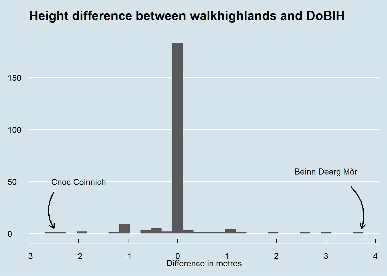
  mutate(height_diff = abs(height_wh - height_dobih),
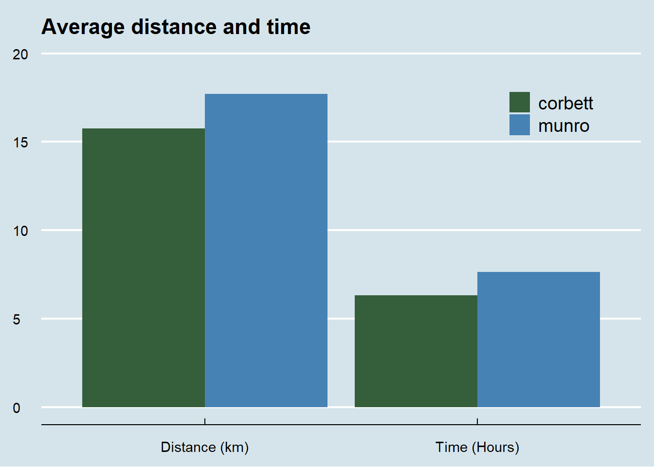
         time = (time_hours_min +time_hours_max)/2,
         type = "corbett") |>
  select(type, "name" = "name_wh",
         region,
         height_wh, height_dobih, height_diff, time,
         first_route_title,, everything(), -name_dobih, -corbett_key_wh, -corbett_key_dobih, -corbett)|>
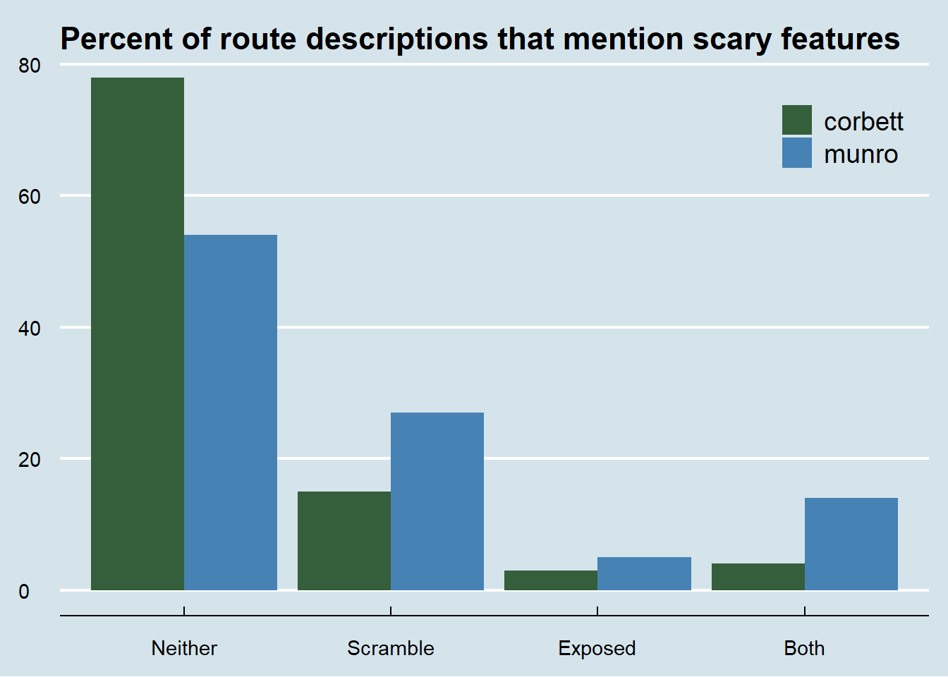
  mutate(scramble_exposed = case_when(
    scramble & exposed ~ "Both",
    scramble & !exposed ~ "Scramble",
    !scramble & exposed ~ "Exposed",
    TRUE ~ "Neither"
  )) |>
  mutate(scramble_exposed = factor(scramble_exposed,
                                   levels = c("Neither", "Scramble", "Exposed", "Both"))) |>
    mutate(wet = case_when(
    spate & bog ~ "Both",
    spate & !bog ~ "Large river",
    !spate & bog ~ "Boggy",
    TRUE ~ "Neither"
  )) |>
  mutate(wet = factor(wet,
                                   levels = c("Neither", "Large river", "Boggy", "Both")))


# make some colour palettes

nature_6 <- c(
  "#355E3B",  
  "#4B4F58",  
  "#4682B4",  
  "#8E6C88",  
  "#E07B39",
  "#BDB76B"
)

nature_5 <- c(
  "#355E3B",  
  "#4B4F58",  
  "#4682B4",  
  "#E07B39",
  "#BDB76B"
)

nature_4 <- c(
  "#355E3B",  
  "#4B4F58",  
  "#4682B4",  
  "#E07B39"   
)

nature_2 <- c(
  "#355E3B",  
  "#4682B4"
)

nature_13 <- c(
  "#355E3B",  # Pine green
  "#6B8E23",  # Moss
  "#BDB76B",  # Dry grass
  "#8B5A2B",  # Earth brown
  "#D2B48C",  # Sand
  "#87CEEB",  # Sky blue
  "#4682B4",  # Loch blue
  "#191970",  # Mountain shadow (midnight blue)
  "#7D7D7D",  # Granite grey
  "#A9A9A9",  # Slate grey
  "#8E6C88",  # Heather purple
  "#E07B39",  # Sunset orange
  "#FFD700"   # Sun yellow
)

nature_11 <- c(
  "#355E3B",  # Pine green
  "#6B8E23",  # Moss
  "#8B5A2B",  # Earth brown
  "#D2B48C",  # Sand
  "#87CEEB",  # Sky blue
  "#4682B4",  # Loch blue
  "#7D7D7D",  # Granite grey
  "#A9A9A9",  # Slate grey
  "#8E6C88",  # Heather purple
  "#E07B39",  # Sunset orange
  "#FFD700"   # Sun yellow
)



nature_19 <- c(
  "#355E3B",  # Pine green
  "#6B8E23",  # Moss
  "#BDB76B",  # Dry grass
  "#8B5A2B",  # Earth brown
  "#D2B48C",  # Sand
  "#87CEEB",  # Sky blue
  "#4682B4",  # Loch blue
  "#191970",  # Mountain shadow (midnight blue)
  "#7D7D7D",  # Granite grey
  "#A9A9A9",  # Slate grey
  "#8E6C88",  # Heather purple
  "#E07B39",  # Sunset orange
  "#FFD700",  # Sun yellow
  "#228B22",  # Forest green
  "#B22222",  # Red clay / bracken
  "#FF69B4",  # Wildflower pink
  "#40E0D0",  # Turquoise (river shallows)
  "#C0C0C0",  # Silver mist
  "#800080"   # Deep purple (moorland heather)
)

# create route data
route_dat <-corbett_dat |>
  select(first_route_url, first_route_title,
         region, time_hours_min:deer_fence, time, scramble_exposed, wet, type) |>
  unique()

route_stats <- corbett_dat |>
  group_by(first_route_title) |>
  summarise(route_rating = janitor::round_half_up(mean(rating), 2),
            route_ascents = janitor::round_half_up(mean(ascents),0 ))

route_dat <- route_dat |>
  left_join(route_stats)

rm(route_stats)

## load in munro dat and combine it

munro_dat <- read_csv("munros_combined.csv")|>
  mutate(type = "munro",
         ycoord = as.character(ycoord))|>
  rename("name" = "munro")

combined_dat <- bind_rows(corbett_dat, munro_dat)|>
  mutate(scramble_exposed = factor(scramble_exposed,
                                   levels = c("Neither", 
                                              "Scramble", 
                                              "Exposed", 
                                              "Both")))

route_dat_combined <-combined_dat |>
  select(first_route_url, first_route_title,
         region, time_hours_min:deer_fence, time, scramble_exposed, wet, type) |>
  unique()

route_stats_combined <- combined_dat |>
  group_by(first_route_title) |>
  summarise(route_rating = janitor::round_half_up(mean(rating), 2),
            route_ascents = janitor::round_half_up(mean(ascents),0 ))

route_dat_combined <- route_dat_combined |>
  left_join(route_stats_combined)

rm(munro_dat, route_stats_combined, walkhighlands)

Height

In my Munro analysis, I originally found that there were some discrepancies between the heights on walkhighlands and the DoBIH (which walkhighlands then corrected, cause they’re great, give them some money) so first, I checked if the same discrepancy existed for the Corbetts.

The short answer is yes. Although the differences are fewer and smaller than for the Munros. Additionally, for the Munros, walkhighlands were always larger whereas there is a mix here and more of them can be explained by rounding.

Show code

corbett_dat <- corbett_dat |>
  mutate(height_diff = height_wh - height_dobih)

ggplot(corbett_dat, aes(x = height_diff)) +
  geom_histogram() +
  theme_economist() +
  scale_x_continuous(breaks = seq(-3,4, 1)) +
  labs(y = NULL, 
       x = "Difference in metres", 
       title ="Height difference between walkhighlands and DoBIH",
       subtitle = "") +
  # labels
    annotate("text",
           x = -2, y = 50,
           label = "Cnoc Coinnich") +
  annotate(geom = "curve", 
          x = -2.5, y = 40, 
          xend = -2.5, yend = 5,
          curvature = 0.3,
          arrow = arrow(length = unit(0.5, "lines")),
          , linewidth = .75)+
  # labels
    annotate("text",
           x = 3, y = 60,
           label = "Beinn Dearg Mòr") +
  annotate(geom = "curve", 
          x = 3.5, y = 45, 
          xend = 3.72, yend = 5,
          curvature = -0.3,
          arrow = arrow(length = unit(0.5, "lines")), linewidth = .75)

Munros vs Corbetts

Rather than just do the same plots for Corbetts as for the Munros I thought it would be interesting to compare the two.

Scary Corbetts

First, I looked at what percent of route descriptions mention scrambling, exposure, both, or neither for Corbetts and Munros. I don’t think it’s particularly surprising that more Munros feature scrambling and exposure but I don’t think I expected the “neither” category to be quite so high for the Corbetts.

Show code

combined_dat |>
  group_by(type) |>
  count(scramble_exposed) |>
  mutate(percent = round_half_up(n/sum(n)*100, 0)) |>
  ungroup() |>
  select(-n) |>
  pivot_wider(names_from = scramble_exposed, values_from = percent) |>
  flextable() |>
  autofit()

Percent of route descruptions that contain scary words
type	Neither	Scramble	Exposed	Both
corbett	78	15	3	4
munro	54	27	5	14

Show code

combined_dat |>
  group_by(type) |>
  count(scramble_exposed) |>
  mutate(percent = round_half_up(n/sum(n)*100, 0)) |>
  ungroup() |>
  select(-n) |>
  ggplot(aes(x = scramble_exposed, y = percent, fill = type)) +
  geom_col(position = "dodge") +
  theme_economist() +
  scale_fill_manual(values = nature_2) +
  labs(x = NULL, y = NULL, fill = NULL, 
       title = "Percent of route descriptions that mention scary features") +
    theme(
    legend.position = "inside",
   legend.position.inside = c(0.9, 0.85),
    legend.text = element_text(size = 14)
  )

There’s far fewer scary Corbetts but it’s good to know where they are - these maps work much better on a full browser than a phone.

Have I mentioned that I dislike heights and exposure?

Show code

corbett_map <- corbett_dat %>%
  select(name, region, xcoord, ycoord, height_dobih, pathless, scramble_exposed, wet, toilet, pub, bothy, deer_fence, car_park) %>%
  na.omit()

# Convert OSGB36 coordinates to sf object
corbett_sf <- corbett_map %>%
  st_as_sf(coords = c("xcoord", "ycoord"), 
           crs = 27700)  # EPSG:27700 is OSGB36 / British National Grid

# Transform to WGS84 (lat/long) for easier plotting
corbett_lat_long <- corbett_sf %>%
  st_transform(crs = 4326)

# Extract coordinates for ggplot
corbett_coords <- corbett_lat_long %>%
  mutate(
    longitude = st_coordinates(.)[,1],
    latitude = st_coordinates(.)[,2]
  ) %>%
  st_drop_geometry() %>%
  arrange(-height_dobih)%>%
  mutate(pathless = factor(pathless,
                           levels = c(FALSE, TRUE),
                           labels = c("Pathed", "Pathless")))


uk_map <- rnaturalearth::ne_countries(scale = "large", 
                                  country = "United Kingdom", 
                                    returnclass = "sf")

# Step 2: Specify shape codes (16 = circle, 17 = triangle, etc.)
shape_values <- c(
  "Neither" = 16,    # filled circle
  "Scramble" = 17,   # filled triangle
  "Exposed" = 15,    # filled square
  "Both" = 18        # filled diamond
)

p <- ggplot() +
  geom_sf(data = uk_map, fill = "lightgray", color = "darkgrey", size = 0.3) +
  coord_sf(xlim = c(-8, -1.5), ylim = c(56.5, 58.6)) +
  geom_jitter(data = corbett_coords, 
             aes(x = longitude, 
                 y = latitude, 
                 shape = scramble_exposed, 
                 colour = scramble_exposed,
                 text = name), 
             size = 1,
             height = .05,
             width = .05) + 
  scale_x_continuous(breaks = NULL) +
  scale_shape_manual(values = shape_values) +
  scale_y_continuous(breaks = NULL) +
  scale_colour_manual(values = nature_4) +
  labs(title = "Where are the scary Corbetts?",
       subtitle = "Walk descriptions that reference:",
       colour = "Route mentions", shape = "Route mentions") +
  theme_economist() +
  theme(
    axis.text = element_blank(),      
    axis.ticks = element_blank(),     
    axis.title = element_blank(),     
    panel.grid = element_blank(),     
    panel.border = element_blank(),
    legend.text = element_text(size = 10)
  )

ggplotly(p, tooltip = "text")

Pathless

This is dedicated to Creag Mac Ranaich and Meall an t-Seallaidh that I bagged last weekend, and to my ankles that only just survived the pathless descent.

A note here that this doesn’t mean the full route is pathless, just that it is mentioned at some point. Additionally, for the map, “Pathed” just means that the route did not mention the word pathless.

Again it’s not a huge surprise that there are more pathless Corbetts but again I didn’t expect the difference to be quite so large.

Show code

combined_dat |>
  group_by(type) |>
  count(pathless) |>
  mutate(percent = round_half_up(n/sum(n)*100, 0)) |>
  ungroup() |>
  select(-n) |>
  filter(pathless == TRUE) |>
  ggplot(aes(x = "", y = percent, fill = type)) +   # <--- "" instead of pathless
  geom_col(position = "dodge") +
  geom_text(aes(label = paste0(percent, "%")), 
            vjust = 2, color = "black", size = 5,
            position = position_dodge(width = 1)) +
  theme_economist() +
  scale_y_continuous(limits = c(0,100)) +
  scale_fill_manual(values = nature_2) +
  labs(x = "Hll type", 
       y = "Percent", 
       fill = NULL, 
       title = "Percent of routes that mention pathless",
       subtitle = "Munro vs Corbett") +
  theme(
    legend.position = "inside",
    legend.position.inside = c(0.9, 0.85),
    legend.text = element_text(size = 14)
  )

Show code

p <- ggplot() +
  geom_sf(data = uk_map, fill = "lightgray", color = "darkgrey", size = 0.3) +
  coord_sf(xlim = c(-8, -1.5), ylim = c(56.5, 58.6)) +
  geom_jitter(data = corbett_coords, 
             aes(x = longitude, 
                 y = latitude, 
                 colour = pathless,
                 text = name), 
             size = 1,
             height = .05,
             width = .05) + 
  scale_x_continuous(breaks = NULL) +
  scale_y_continuous(breaks = NULL) +
  scale_colour_manual(values = nature_2) +
  labs(title = "Where are the pathless Corbetts?",
       subtitle = "Walk descriptions that reference:",
       colour = NULL) +
  theme_economist() +
  theme(
    axis.text = element_blank(),      
    axis.ticks = element_blank(),     
    axis.title = element_blank(),     
    panel.grid = element_blank(),     
    panel.border = element_blank(),
    legend.text = element_text(size = 10)
  )

ggplotly(p, tooltip = "text")

Distance and length

These analyses are done using the route data rather the individual hills (because some routes have more than one hill). That the Munros routes are longer in both distance and time is not a surprise but in this case, I think I might have expected the difference to be larger than it is and also, the longest route on walkhighlands is a Corbett, not a Munro. Don’t underestimate the Corbetts!

Show code

route_dat_combined |>
  group_by(type) |>
  summarise(distance = round(mean(distance_km),2),
            time = round(mean(time),2)) |>
  flextable()

Mean route distance (km) and time (hours) by hill type
type	distance	time
corbett	15.77	6.31
munro	17.70	7.63

Show code

route_dat_combined |>
  group_by(type) |>
  summarise(distance = mean(distance_km),
            time = mean(time)) |>
  pivot_longer(cols = distance:time,
               names_to = "measurement", 
               values_to = "values") |>
  ggplot(aes(x = measurement, y = values, fill = type)) +
  geom_col(position = "dodge") +
  scale_fill_manual(values = nature_2) +
  theme_economist() +
  scale_x_discrete(labels = c("Distance (km)", "Time (Hours)")) +
  scale_y_continuous(limits = c(0, 20)) +
  labs(x = NULL, y = NULL, title = "Average distance and time",
       fill = NULL)+
  theme(strip.text = element_blank(),
        legend.position = "inside",
        legend.position.inside = c(.85, .8),
        legend.text = element_text(size = 14))

I no-one cares but these arrows took me bloody ages.

Show code

labels <- tibble::tribble(
  ~type,     ~x,   ~y,   ~label,
  "munro",    2,   26,  "Meall Buidhe",
  "munro",   16,   28,  "Lurg Mhòr\n& Bidein a' Choire Sheasgaich",
  "corbett",  -1,   38,  "Meall nam Maigheach\n/ Sgùrr a' Chaorachain",
  "corbett", 15,   32,  "Beinn a' Chlaidheimh"
)

arrows <- tibble::tribble(
  ~type,     ~x,   ~y,   ~xend, ~yend, ~curve,
  "munro",    3,   23,    3,     5,    0.3,
  "munro",   16,   20,   16,     5,   -0.3,
  "corbett",  0,   28,    2,   5,    0.3,
  "corbett", 15,   25,   15,     5,   -0.3
)

ggplot(route_dat_combined, aes(x = time, fill = type)) +
  geom_histogram(binwidth = 1, colour = "black") +
  facet_wrap(~type, nrow = 2) +
  scale_x_continuous(breaks = seq(0, 18, 1)) +
  theme_economist() +
  labs(x = "Length of walk in hours", 
       y = "Count", 
       title = "Munros vs Corbetts",
       subtitle = "Length of walk (hours)",
       fill = NULL) +
  scale_fill_manual(values = nature_2) +
  theme(strip.text = element_blank(),
        legend.position = "inside",
        legend.position.inside = c(.9, 1),
        legend.text = element_text(size = 14)) +

  # curves with curvature = 0.3
  geom_curve(data = arrows %>% filter(curve > 0),
             aes(x = x, y = y, xend = xend, yend = yend),
             inherit.aes = FALSE,
             curvature = 0.3,
             arrow = arrow(length = unit(0.5, "lines")),
             linewidth = .75) +

  # curves with curvature = -0.3
  geom_curve(data = arrows %>% filter(curve < 0),
             aes(x = x, y = y, xend = xend, yend = yend),
             inherit.aes = FALSE,
             curvature = -0.3,
             arrow = arrow(length = unit(0.5, "lines")),
             linewidth = .75) +

  # labels
  geom_text(data = labels,
            aes(x = x, y = y, label = label,
                hjust = ifelse(x > 10, 1, 0)),
            inherit.aes = FALSE, size = 3.5)

Show code

labels <- tibble::tribble(
  ~type,     ~x,   ~y,   ~label,
  "munro",    1,   18,  "Ben Hope\n/ Sgùrr na Banachdich",
  "munro",  42,   12,  "An Scarsoch and\nCàrn an Fhìdhleir",
  "corbett",  4.5,   20,  "Beinn Luibhean",
  "corbett", 45,   15,  "Beinn a' Chaisgein Mòr"
)

arrows <- tibble::tribble(
  ~type,     ~x,   ~y,   ~xend, ~yend, ~curve,
  "munro",    5,  14,   6.75,     3,    0.3,
  "munro",   40,   8,   42,     2,   -0.3,
  "corbett",  4.5,  18,    4,   2,    0.3,
  "corbett", 40,   13,   45,     2,   -0.3
)


ggplot(route_dat_combined, aes(x = distance_km, fill = type)) +
  geom_histogram(binwidth = 1, colour = "black") +
  facet_wrap(~type, nrow = 2) +
  scale_x_continuous(breaks = seq(0, 50, 5)) +
  theme_economist() +
  labs(x = "Length of walk in km", 
       y = "Count", 
       title = "Munros vs Corbetts",
       subtitle = "Length of walk (km)",
       fill = NULL) +
  scale_fill_manual(values = nature_2) +
  theme(strip.text = element_blank(),
        legend.position = "inside",
        legend.position.inside = c(.9, 1),
        legend.text = element_text(size = 14)) +

  # curves with curvature = 0.3
  geom_curve(data = arrows %>% filter(curve > 0),
             aes(x = x, y = y, xend = xend, yend = yend),
             inherit.aes = FALSE,
             curvature = 0.3,
             arrow = arrow(length = unit(0.5, "lines")),
             linewidth = .75) +

  # curves with curvature = -0.3
  geom_curve(data = arrows %>% filter(curve < 0),
             aes(x = x, y = y, xend = xend, yend = yend),
             inherit.aes = FALSE,
             curvature = -0.3,
             arrow = arrow(length = unit(0.5, "lines")),
             linewidth = .75) +

  # labels
  geom_text(data = labels,
            aes(x = x, y = y, label = label,
                hjust = ifelse(x > 10, 1, 0)),
            inherit.aes = FALSE, size = 3.5)

User ratings

Which region has the highest and lowest rated Corbetts (by user rating)? The bottom three are the same for the Munros but the top three are a little different - for Munros Isle of Skye, Torridon, and Fort William took the podium whereas Ullapool and Sutherland claim their place for Corbetts.

Show code

region_rating <- corbett_dat |>
  group_by(region) |>
  summarise(avg_rating = mean(rating, na.rm = TRUE), 
            n = n(),
            .groups = "drop") |>
  filter(n >= 5)


ggplot(
  semi_join(corbett_dat, region_rating, by = "region"),
  aes(
    x = rating,
    y = fct_reorder(region, rating, .fun = mean, .desc = FALSE),
    fill = region
  )
)  +
  geom_density_ridges(
    quantile_lines = TRUE, quantile_fun = mean,
    vline_linetype = "dashed",
    aes(colour = "Mean height (m)")
  ) +
  scale_y_discrete(expand = c(0.01, 0)) +
  scale_x_continuous(expand = c(0.01, 0)) +
  scale_colour_manual(values = c("Mean height (m)" = "black")) +
  theme_economist() +
  scale_fill_manual(values = nature_11) +
  labs(
    x = NULL, y = NULL,
    title = "User ratings by region",
    colour = NULL,
    subtitle = "Regions w/ 5+ Corbetts"
  ) +
  guides(fill = "none") +
  theme(
    legend.position = "inside",
   legend.position.inside = c(0.87, 1.1),
    legend.text = element_text(size = 10)
  )+
  theme(
    plot.title.position = "plot",                
    plot.title = element_text(margin = margin(b = 10)))

And here’s the full list in table form (the graphs only have those regions with 5 or more Corbetts, they are a lot of regions that have fewer than this):

Show code

#| tbl-cap: "Mean Corbett user rating by region"

corbett_dat |>
  group_by(region) |>
  summarise(avg_rating = mean(rating, na.rm = TRUE), 
            "no. corbetts" = n(),.groups = "drop") |>
  arrange(desc(avg_rating)) |>
  flextable() |>
  colformat_double(digits = 2)|>
  autofit()

region	avg_rating	no. corbetts
Isle of Rum	4.66	2
Isle of Arran	4.55	4
Outer Hebrides	4.41	1
Islay, Jura and Colonsay	4.32	1
Skye	4.23	2
Torridon	4.17	19
Isle of Mull	4.11	1
Ullapool	3.92	17
Sutherland	3.91	10
Fort William	3.69	55
Loch Lomond	3.60	17
Dumfries and Galloway	3.54	6
Kintail	3.52	10
Argyll	3.43	12
Loch Ness	3.29	11
Moray	3.26	2
Perthshire	3.17	24
Cairngorms	3.12	24
Angus	3.05	3
Borders	2.95	1

Bothy plot

I didn’t see the point in mapping all the non-natural features like I did for the Munros but given there’s quite a few long Corbett routes, a bothy plot is of use.

Show code

bothy_plot <- ggplot() +
  geom_sf(data = uk_map, fill = "lightgray", color = "darkgrey", size = 0.3) +
  coord_sf(xlim = c(-8, -1.5), ylim = c(56, 58.6)) +
  geom_jitter(data = filter(corbett_coords, bothy == TRUE), 
             aes(x = longitude, 
                 y = latitude, 
                 colour = bothy,
                 text = name), 
             size = 1) + 
  scale_x_continuous(breaks = NULL) +
  scale_y_continuous(breaks = NULL) +
  labs(title = "Corbett routes that mention a bothy") +
  guides(colour = "none") +
  theme_economist() +
  theme(
    axis.text = element_blank(),      
    axis.ticks = element_blank(),     
    axis.title = element_blank(),     
    panel.grid = element_blank(),     
    panel.border = element_blank(),
    legend.text = element_text(size = 10)
  )

ggplotly(bothy_plot, tooltip = "text")

Ascents by rating

Number of ascents (how many people have recorded on walkhighlands that they have bagged a particular Corbett ) by ratings

Show code

p <- ggplot(route_dat, aes(x = route_ascents, y = route_rating)) +
  geom_point(aes(text = first_route_title)) +
  theme_economist() +
  scale_y_continuous(breaks = seq(1:5)) +
  scale_x_continuous(breaks = seq(0, 12000, 2000))+
  coord_cartesian(ylim = c(1,5)) +
  labs(y = "User rating (1-5)",
       x = "Number of recorded ascents",
       title = "Number of ascents by rating")

p +
  annotate(geom = "curve", 
          x = 10500, y = 3, 
          xend = 11437, yend = 4.4,
          curvature = 0.3,
          arrow = arrow(length = unit(0.5, "lines")),
          linewidth = .75) +
    annotate("text",
           x = 10500, y = 2.8,
           label = "The Cobbler ") +
    annotate(geom = "curve", 
          x = 9200, y = 4.6, 
          xend = 8976, yend = 4.1,
          curvature = -0.3,
          arrow = arrow(length = unit(0.5, "lines")),
          linewidth = .75) +
    annotate("text",
           x = 8976, y = 4.8,
           label = "Ben Ledi")+
    annotate(geom = "curve", 
          x = 7329, y = 3.5, 
          xend = 7329, yend = 3.9,
          curvature = -0.3,
          arrow = arrow(length = unit(0.5, "lines")),
          linewidth = .75) +
    annotate("text",
           x = 7329, y = 3.3,
           label = "Ben Vrackie")+
    annotate(geom = "curve", 
          x = 6000, y = 4.6, 
          xend = 6800, yend = 4.4,
          curvature = 0.3,
          arrow = arrow(length = unit(0.5, "lines")),
          linewidth = .75) +
    annotate("text",
           x = 6000, y = 4.7,
           label = "Goat Fell")

And here’s that as an interactive map so you can see them all.

Show code

ggplotly(p, text = first_route_title)

Rating by feature

It’s not a surprise to me that scrambling routes are higher rated, but it is a surprise that across the board, Corbett routes are rated higher than Munros. My suspicion is that it is a combination of more people rating the Munros, and the enthusiasm for hills of the people who are likely to walk them.

Show code

route_dat_combined |>
  group_by(type, scramble_exposed) |>
  summarise(rating = mean(route_rating)) |>
  ggplot(aes(x = scramble_exposed, y = rating, fill = type)) +
  geom_col(position = "dodge") +
  scale_fill_manual(values = nature_2) +
  theme_economist() +
  labs(x = NULL, 
       y = NULL, 
       fill = NULL, 
       title = "User ratings by scary features") +
  coord_cartesian(ylim = c(0,5))+
    theme(
    legend.position = "inside",
   legend.position.inside = c(0.1, 0.85),
    legend.text = element_text(size = 14)
  )